Tag Archives: visualization

Know Your MP: Probing Election Affidavits with Maps

Project by Shailendra Paliwal and Kashmir Sihag
Note: This blog post was written by Shailendra

I want to share a 3 year old project I and my friend Kashmir Sihag Chaudhary did for Jaipur Hackathon in a span of 24 hours. It is called Know Your MP, it visualizes data that we know about our members of parliament on a map of Indian Parliamentary Constituencies.

A friend and a fellow redditor Shrimant Jaruhar had already made something very similar in 2014 but it was barely usable since it took forever to load and mostly crashed my browser. My attempt with Know Your MP was to advance on the same idea.

The Dataset

Election Commission of India requires that every person contesting the elections fill an affidavit and therby disclosing criminal, financial and educatinal background of each candidate. There have been a few concerns about this, a major one being that one could as well enter misleading information without any consequences. If you would remember the brouhaha over education qualifications of Prime Minister Modi and the cabinet minister Smriti Irani, it started with what they entered in their election affidavits. However, it is widely believed that a vast majority of the data colllected is true or close to true which makes this a dataset worthy of exploration.

However, like a lot of data from governments, every page from these affidavits are made available as individual images behind a network of hyperlinks on the website of Election Commission of India. Thankfully, all of this data is available as CSV or Excel Spreadsheets from [MyNeta.info](http://myneta.info/). The organization behind MyNeta is Association of Democratic Reforms(ADR) which was established by a group of professors from Indian Institute of Management (Ahmedabad). ADR also played a pivotal role in the Supreme Court ruling that brought this election disclosure to fruition.

everything is neatly laid out


Cadidate Affidavit of CPI(M) candidate Udai Lal Bheel from Udaipur Rural constituency in Rajasthan. link

Preparing the Map

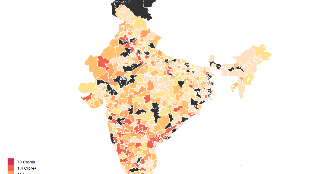
This data needs to be visualized on a map with boundaries showing every parliamentary contituency. Each constituency will indicate the number of criminal cases or assets of their respective MP using a difference in shading or color. Such visualizations are called choropleth maps. To my surprise, I couldn not find a map of Indian parliamentary constituencies from any direct or indirect government sources. That is when datameet came to my rescue. I found that DataMeet Bangalore had released such a shapefile. It is a 13.7MB file(.shp). Certainly not usable for a web project.

Next task would be somehow compress this shapefile to a small enough size that can be then used either as a standalone map or as an overlay on leaflet.js or Google Maps (or as I later learned Mapbox too).

From the beginning I was looking at d3.js to achieve this. The usual process to follow would be to convert the shapefile (.shp) into JSON format which D3 can use.

For map compression I found that Mike Bostock (a dataviz genius and also the person behind D3) has worked on a map format that does such compression, the format is called GeoJSON. After a bit of struggling with making things work on a Windows workstation and tweaking around with the default settings, I managed to bring the size down to 935 KB. Map was now ready for the web and I now had to only wade through D3 documentation to make the visualization.

Linking data with map and Visualization

Each parliamentary region in the GeoJSON file has a name tag which links it to the corresponding data values from dataset. A D3 script on the HTML page parses both and does this job to finally render this choropleth map.

The black regions on the maps are parliamentary contituencies that have alternate spellings. I could have used levenshtein distance to match them or more simply linked the map to data with a numeric ID. I’ll hopefully get that done someday soon.

link to project, github, map

Finally Looking at Data

The average member of parliment (only a few MPs have changed since 2015) has at least 1 criminal case against them, has a total asset value of about 14 Crore INR and has liabilities of value 1.4 Crore INR. But this dataset also has a lot of outliers so mean isn’t really the best representative of the central tendency. The median member of parliament has 0 criminal case against them, has total assets worth 3.2 Crore INR and has liabilities of value 11 Lakh INR.

The poorest member of parliament is Sumedha Nand Saraswati from Sikar who has total assets worth 34 thousand INR. Richest MP on the other hand is Jayadev Galla with declared assets of 683 Crore INR. Galla doesn’t directly fit the stereotypical corrupt politician meme with zero criminal cases against him. His wealth is best explained to the success of lead acid battery brand Amaron owned by the conglomerate his father founded in 1985.

Making A Football Data Viz With D3 and Reveal.js

This is a write-up on how I made a slideshow for the Under-17 World Cup.

The U-17 World Cup is the first-ever FIFA tournament to be hosted by India. Like many of you, I’ve seen plenty of men’s World Cups, but never an U-17 one. To try and understand how the U-17 tournament might be different from the ‘senior’ version, I compared data from the last U-17 World Cup held in Chile in 2015 and the last men’s World Cup in Brazil in 2014.

The data was taken from Technical Study Group reports that are published by FIFA after every tournament. (The Technical Study Group is a mixture of ex-players, managers and officials associated with the game. You can read more about the group here.)

In particular, I used the reports for the 2014 World Cup and the 2015 U-17 World Cup. The data was taken pretty much as is, and thankfully didn’t have to be processed much. An example of the data available in the report can be seen in the image below. It shows how the 171 goals in the 2014 World Cup came about.

A look at some of the data in the report

The main takeaway from the comparison with the men’s World Cup is that the U-17 World Cup might see more goals and fewer 0-0 draws on average. The flipside is that there could be more cards and penalties too. For more details, check the slideshow.

BE LESS INTIMIDATING FOR READERS

I know just using one World Cup each to represent men’s and U-17 football may not be particularly rigorous. We could have also used data from the previous three or four World Cups in each age format. But if I did that, I was scared the data story would become more dense and intimidating for readers. I wanted to make this easy to follow along and understand, which is why I simplified things this way.

A card from the slideshow

Another thing I did to make this easier to digest was to stick to one main point per card (see image above). The main point is in the headline, then you get a few lines of text below showing how exactly you’ve arrived at the main point. The figures that have been calculated and compared are put in a bold font. Then there is an animated graphic below that, which visually reinforces the main point of the slide.

The data story tries to simulate a card format, one that you can just flick through on the mobile. I used the slideshow library reveal.js to make the cards. But I suspect there is a standard, more established method that mobile developers have to create a card format, will have to look into this further.

The animations were done with D3.js, with help from a lot of examples on stackoverflow and bl.ocks.org. If you’re new to D3 and want to know how these animations were done, here’s more info.

ANIMATING THE BAR CHART

The D3 ‘transitions’ or animations in this slideshow are basically the same. There’s (a) an initial state where there’s nothing to see, (b) the final state where the graphic looks the way you want and (c) a transition from the initial state to the final state over a duration specified in milliseconds.

A snippet of code for animating the bars

For example, in the code snippet for the bar animation above, you see two attributes changing for the bars during the transition—the ‘height’ and ‘y’ attributes changing over a duration of 500 milliseconds. You can see another example of this animation at bl.ocks.org here.

ANIMATING THE STACKED BAR CHART

This animation was done in a way similar to the one above. The chart is called a ‘normalised stack chart’ and the code for this was taken from the bl.ocks.org example here.

The thing about this chart is that you don’t have to calculate the percentages beforehand. You just feed in the raw data (see image below) and you get the final percentages visualised in the graphic.

The raw data on goals gets converted to percentages

ANIMATING THE LINE CHART

The transition over here isn’t very sophisticated. In this, the two lines and the data points on them are basically set to appear 300 milliseconds and 800 milliseconds respectively after the card appears on screen (see the code snippet below).

A snippet of code for changing the opacity of the line

A cooler line animation would have been ‘unrolling’ the line as seen in this bl.ock.org example. Maybe next time!

ANIMATING THE PIE CHART

Won’t pretend to understand the code used here. I basically just adapted this example from bl.ocks.org and played around with the parameters till it came out the way I wanted. This example is from Mike Bostock, the creator of D3.js, and in it he explains his code line by line (see image below). Do look at it if you want to fully understand how this pie chart animation works.

Commented code from Bostock

ANIMATING THE ISOTYPE CHART

Yup, this chart is called an isotype chart. This animation is another one where the transition uses delays. So if you look in the gif, you see on the left side three cards being filled one after the other.

Some of the code used in animating this isotype chart

They all start off with an opacity of 0, which makes them invisible (or transparent, technically). What the animation does is make each of the cards visible by changing the opacity to 1 (see image above). This is done after different delay periods of 200 milliseconds for the bottom card, 400 for the card in the middle and 600 milliseconds for the card on top.

FINAL WORD

If you’ve never worked with D3 before, hope this write-up encourages you to give it a shot. You can look at all the code for the slideshow in the github repo here. All comments and feedback are welcome! 🙂

COVER IMAGE CREDIT: Made in inkscape with this picture from Flickr